When one particular species of event has always … been conjoined with another,
we make no longer any scruple of foretelling one upon the appearance of the other,
and of employing that reasoning, which can alone assure us of any matter of fact or existence.
We then call the one object, Cause; the other, Effect.
- David Hume's (1748, §7) An Enquiry Concerning Human Understanding
Rubin Causal Model
|
|||||||||||||||||||||
|---|---|---|---|---|---|---|---|---|---|---|---|---|---|---|---|---|---|---|---|---|---|

|
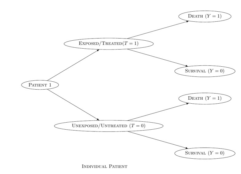
The Rubin Causal Model is also known as the Neyman-Rubin Causal Model or Potential Outcomes Approach According to the Rubin Causal Model (Neyman, 1923, Rubin, 1974, Holland & Rubin, 1983, Robins, 1986, Hernán & Robins, 2020): A treatment T has a causal effect on the healthcare outcome Y, if there is a difference between the two potential outcomes YT = 0 and YT = 1 Otherwise, T has no causal effect on Y
The fundamental problem of causal inference:
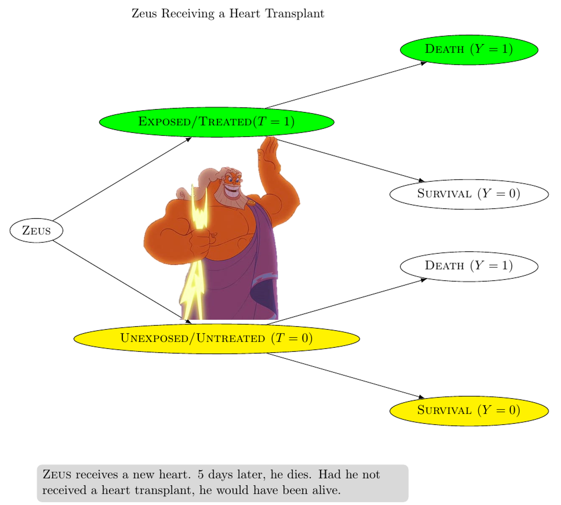
In EXAMPLE 1, Zeus receives a heart transplant (T = 1) 5 days later, Zeus dies (Y = 1) Had Zeus not received a heart transplant, he would have been alive (i.e. YT = 0 = 0) 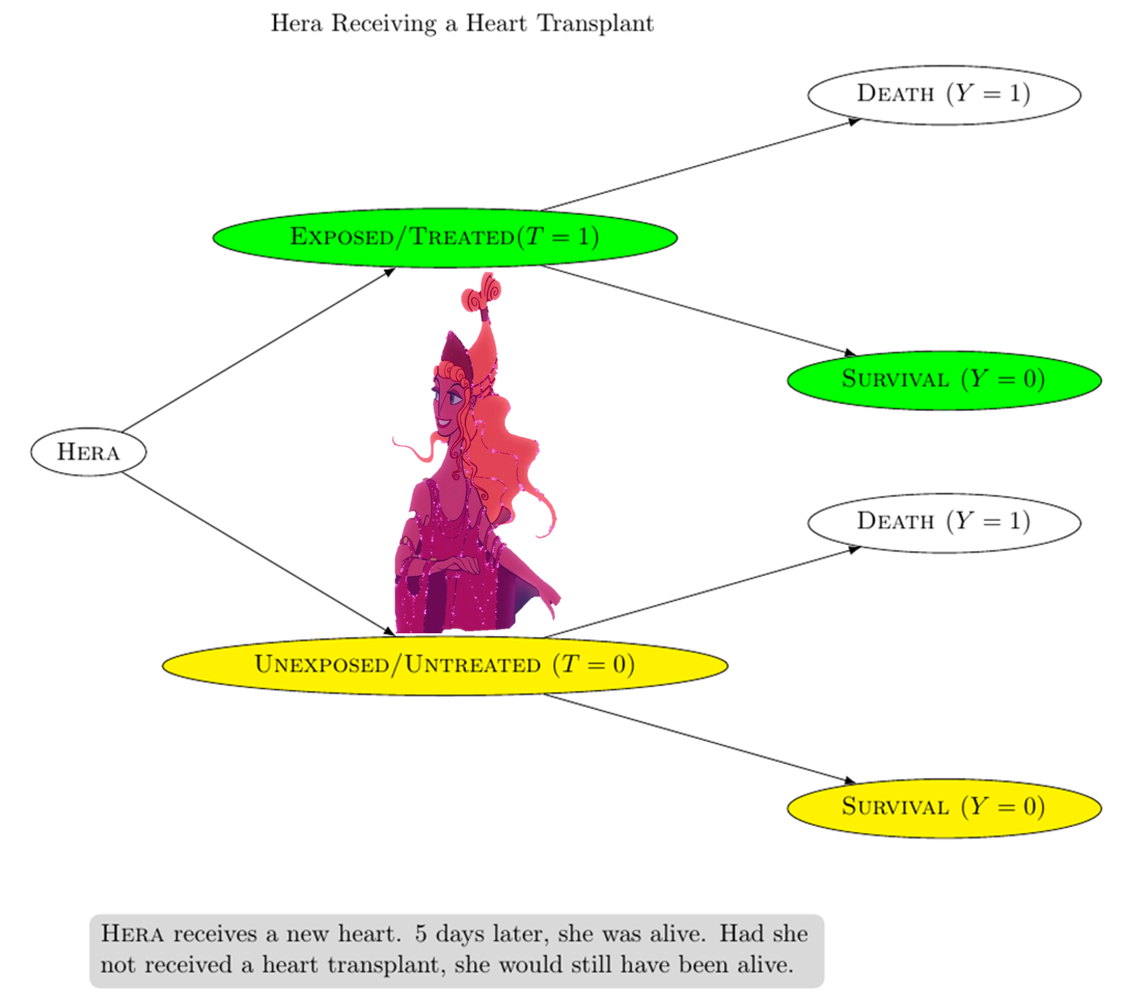
In EXAMPLE 2, Hera receives a heart transplant (T = 1) 5 days later, Hera is still alive (Y = 0) Had Hera not received a heart transplant, she would still have been alive (i.e. YT = 0 = 0) From EXAMPLE 1 and EXAMPLE 2: The actual outcome for Zeus is death (Y = 1) and the counterfactual outcome for Zeus is survival (YT = 0 = 0) The actual outcome for Hera is survival (Y = 0) and the counterfactual outcome for Hera is survival (YT = 0 = 0) If the two outcomes (actual and counterfactual) differ, then we say that the treatment T has a causal effect on the healthcare outcome Y Otherwise, T has no causal effect on the healthcare outcome ∴ CONCLUSION 1: The heart transplant caused Zeus' death ∴ CONCLUSION 2: The heart transplant had no causal effect on Hera's survival Reasoning in terms of counterfactuals provides the basis of causal inference Compare with the counterfactual theory of causation Well-defined counterfactuals are necessary for meaningful causal inference (Robin & Greenland, 2000) |
||||||||||||||||||||

|
Suppose that we conduct a 20-person study about the effectiveness of a treatment This 20-person study would be too small for us to reach any definite conclusions Random fluctuations arising from sampling variability could explain almost anything Nonetheless, we could assume that each individual in our population represents 1 billion individuals who are identical to him or her ∴ We would end up with a super-population of 20 billion individuals 
ASSUMPTION 1 (Pre-modelling): Individual counterfactual outcomes are deterministic We could imagine a scenario in which the counterfactual outcomes are stochastic rather than deterministic w.r.t. an individual Perhaps this individual's probability of dying under treatment (0.9) and under no treatment (0.1) are neither zero nor 1 Nonetheless, our statistical estimates and confidence intervals for causal effects in the super-population are identical, irrespective of whether the world is stochastic (quantum) or deterministic (classical) at the level of individuals ASSUMPTION 2 (Pre-modelling): No interference — also known as 'no interference between units' (Cox, 1958) or the 'stable-unit-treatment-value assumption (SUTVA)' (Rubin, 1980) An individual's counterfactual outcome under a certain treatment value does not depend on the treatment values of other individuals ASSUMPTION 2 would be less feasible in studies where interference between individuals is common (e.g. studies dealing with contagious agents) ASSUMPTION 3 (Pre-modelling): Mortality Death is delayed, not prevented, by the treatment |
||||||||||||||||||||

Image source: Eric Sucar |
ASSUMPTION 1 (Modelling): Consistency In the actual world, Zeus was treated (T = 1) According to ASSUMPTION 1, Zeus' counterfactual outcome under treatment (YT = 1 = 1) is equal to his observed outcome Y = 1 More generally, Yt = Y for every individual with T = t, where t corresponds to an individual's observed treatment value The two main COMPONENTS of ASSUMPTION 1 are:
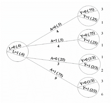
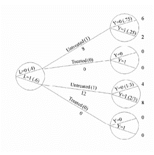
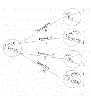
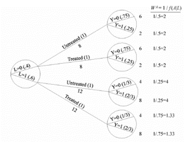
ASSUMPTION 2 (Modelling): Exchangeability Exchangeability means that the actual treatment and the counterfactual outcome are independent Exchangeability is defined as the independence between the counterfactual outcome YT and the observed treatment T When the treated and untreated are exchangeable, we say that the treatment is exogenous Formally: YT ⫫ T NOTE: Exchangeability does not imply independence between the observed outcome and the observed treatment YT ⫫ T is mathematically distinct from Y ⫫ T Conditional exchangeability: YT ⫫ T | L, where L denotes the measured covariates (e.g. L = 1 for patients in a critical condition and L = 0 for patients in a non-critical condition) If YT ⫫ T | L, then the treated and untreated are conditionally exchangeable within the levels of variable L If YT ⫫ T | L, then the conditional probability of receiving every value of treatment depends only on the measured covariates L ASSUMPTION 3 (Modelling): Positivity — also known as the 'experimental treatment assumption' The probability of receiving every value of treatment, conditional on L, is greater than zero ∴ Under ASSUMPTION 3, there are patients at all levels of treatment (e.g. T = 0, T = 10 in every level of L (e.g. L = 0, L = 1) Formally: P(T = t|L = l) > 0 for all values of l, with P(L = l) ≠ 0 in the population of interest If doctors always transplant a heart (T = 1) to individuals in a critical condition (L = 1), then ASSUMPTION 3 would not hold P(T = 0|L = 1) = 0 ASSUMPTION 1 (Consistency), ASSUMPTION 2 (Exchangeability), and ASSUMPTION 3 (Positivity) are jointly referred to as the identifiability conditions or assumptions |
||||||||||||||||||||


|
Randomized experiments are the gold standard and real-world data can be used for causal inference if we conduct randomized experiments The randomized assignment of treatment leads to exchangeability In a marginally randomized experiment, we use a single unconditional marginal randomization probability Randomized controlled trials (RCTs) are supported by Fisher's (1925) theory of experimental design EXAMPLE 1: We may flip a single coin to determine whether to assign treatment to each individual EXAMPLE 2: We may randomly select 65 patients for treatment However, it is often infeasible or impossible to conduct marginally randomized experiments A conditionally randomized experiment is a combination of two or more separately marginally randomized experiments EXAMPLE 1: A conditionally randomized experiment may be constituted by a combination of two experiments E1 and E2 E1 is conducted w.r.t. the subset of individuals in critical condition (L = 1) E2 is conducted w.r.t. the subset of individuals in non-critical condition (L = 0) ∴ In the subset of individuals in critical condition (L = 1), the treated and untreated are exchangeable ∴ In the subset of individuals in non-critical condition (L = 0), the treated and untreated are exchangeable Observational studies are less convincing because they lack randomized treatment assignment However, causal inference from observational data is more plausible if we have grounds for regarding an observational study as a conditionally randomized experiment Recall how ASSUMPTION 1 (Consistency), ASSUMPTION 2 (Exchangeability), and ASSUMPTION 3 (Positivity) constitute the identifiability conditions If the identifiability conditions (viz. ASSUMPTIONS 1-3) hold, then we can maintain an analogy between observational study and conditionally randomized experiments This will allow us to identify causal effects from observational data However, whenever any of the identifiablity conditions does not hold, the analogy between observational study and conditionally randomized experiments breaks down (Hernán & Robins, 2020) |
||||||||||||||||||||

|
|
||||||||||||||||||||

|
|
||||||||||||||||||||
Background image taken from: https://cdn.asiatatler.com/asiatatler/i/th/2020/02/04101225-aurora-1185464-1920_cover_1920x1280.jpg This website has been coded using html, css, and js and is dedicated to B and H .