When one particular species of event has always … been conjoined with another,
we make no longer any scruple of foretelling one upon the appearance of the other,
and of employing that reasoning, which can alone assure us of any matter of fact or existence.
We then call the one object, Cause; the other, Effect.
- David Hume's (1748, §7) An Enquiry Concerning Human Understanding
Kleinberg Causal Model
Causal Hierarchy
Three-level causal hierarchy
Three-level causal hierarchy
Level
Syntax
LEVEL 1 (lowest): Association
NOTE: Association involves purely statistical relationships, defined by pure data
P(Y = y|X = x)
TRANSLATION: The conditional probability that Y has the value y, given that we have observed that X has the value x
LEVEL 2 (intermediate): Intervention
NOTE: Intervention involves not just seeing what there is, but changing what we see
P(Y = y|do(X = x), Z = z)
TRANSLATION: The conditional probability that Y has the value y, given that we intervene and set the value of X to x and observe that Z has the value z
TRANSLATION: The conditional probability that Y = y would have been observed had X taken the value x, given that we actually observed X to take the value x′ and Y the value y′
A causal model that is sufficiently representative will cover all these levels in the causal hierarchy
Depending on how accurately the system is represented, common causes may not always render their effects independent
EXAMPLE from Spirtes et al (2000):
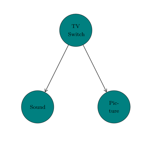
Conjunctive Fork
When the TV does turn on, both the sound and the picture turn on too
∴ The TV switch is a common cause of the sound and the picture
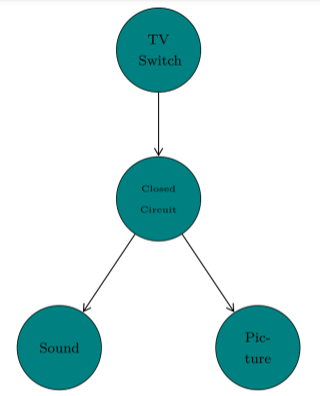
Interactive Fork
However, the TV switch does not always turn the TV on
∴ The picture is not independent on the sound, when conditioned on the state of the TV switch
∴ The CMC is violated
Nonetheless, we can resolve the issue by adding a variable to indicate when there is a closed circuit
Conjunctive forks and interactive forks could be indistinguishable observationally and experimentally
In this EXAMPLE, we still need common knowledge about how circuits work to resolve the issue
More generally, the CMC is perhaps the most debated portion of the Pearl Causal Model
There is much critique about the CMC (Cartwright, 2001, 2002, Freedman & Humphreys, 1999; Humphreys & Freedman, 1996)
Others have conversely defended the CMC (Hausman & Woodward, 1999, 2004)
As the CFC is defined w.r.t. the true probability distribution, we expect the CFC to be true only in a large sample limit
With insufficient data, observations cannot be assumed to be indicative of true probabilities
However, the CFC could be violated even with sufficient data
This is beacuse a variable might be connected by multiple causal paths to another variable
∴ We could have distributions where these multiple paths exactly cancel out so that the cause seems to have no impact on the effect
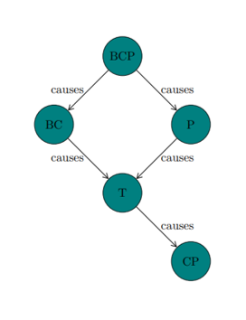
BCP (birth control pills) acts through multiple paths w.r.t. T (thrombosis)
∴ Where these multiple paths between BCP and T exactly cancel out, the CFC would be violated
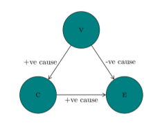
Here is another EXAMPLE in which the CFC could be violated:
Smoking (C) is a positive cause of lung cancer (E)
Living in the country (V) is a positive cause of smoking (C): due to cleaner air in the country, country-dwellers feel freer to smoke
Living in the country (V) is a negative cause of lung cancer (E), due to lack of air pollution
∴ Due to the multiple paths between V and E, the CFC could again be violated under certain circumstances
One of the most important pieces of temporal information is the time it takes for the cause to produce the effect
However, the Pearl Causal Model does not incorporate temporal information
1st CONSEQUENCE: Difficulty in answering policy-oriented questions
Temporal information is useful for policy- or use-related questions (see Cartwright, 2007)
Policy decisions may vary considerably with the length of time between cause and effect
2nd CONSEQUENCE: Over-reliance on background knowledge
The Pearl Causal Model relies on background or mechanistic knowledge (typically from human experts) to find the temporal ordering of relationships
However, such background or mechanistic knowledge might not always be available
PROBLEM 5: Insufficiently Expressive
DAGs (on which the Pearl Causal Model relies) are directed acyclic graphs: they do not admit cycles
However, many systems (specifically: biological systems) have cyclic patterns that repeat over a long trace
The Pearl Causal Model ignores feedback loops and cycles and is unable to infer causal relationships that take the form of feedback loops and cycles
The Wiener-Granger causality approach infers Granger-causality relationships from a set of time-series data
The Pearl Causal Model infers causal relationships from DAGs (causal graphs) and NPSEMs (causal equations) that are generated relative to a dataset
The Kleinberg Causal Model infers causal relationships from a set of time-series data and employs Probabilistic Computation Tree Logic and Kripke structures (causal diagrams)
Probabilistic Computation Tree Logic (PCTL)
Components
Description
Propositional variables
p, q, r, …
Logical connectives
∼ — negation
∧ — conjunction
∨ — inclusive disjunction
→ — material conditional
⟷ — material biconditional
Path quantifiers (see Clarke, Emerson, & Sistla, 1986)
NOTE: Path quantifiers describe whether a property holds for ALL paths (A) or for some path (E), starting at a given state
A — for all paths (similar to ∀ ('for all'))
E — at least one path (similar to ∃ ('there exists at least one'))
NOTE: Path formulae are true or false along a specific path
Monadic temporal operators
F — eventually (i.e. finally or eventually, at some state on the path, the property will hold)
G — always (i.e. globally or always, along the entire path, the property will hold)
X — at the next state of the path, the property will hold
Dyadic temporal operators
U — until (i.e. for two properties, the 1st holds at every state along the path until at some state the 2nd property holds)
W — weak until (i.e. for two properties, the 1st holds at every state along the path until a state where the 2nd property holds, with no guarantee that the 2nd property will ever hold (in which case the 1st property must remain true forever))
NOTE: Path quantifiers and temporal operators (monadic or dyadic) must be paired
Possible pairs of path quantifiers and temporal operators: AF, EF, AG, EG, AX, EX, AU, EU, AW, EW
μ
tp denotes a probability measure on a set of paths, such that:
i) t (for time) is a non-negative integer or ∞
ii) p (for probability) is a real number such that 0 ≤ p ≤ 1
Temporal logic (CTL, PCTL, etc) is usually interpreted in terms of Kripke structures
A Kripke structure M over AP is the 4-tuple M = { S, S0, R, L }, where:
AP is a set of atomic propositions;
S is a finite set of states;
S0 ⊆ S is the set of initial states;
R ⊆ S × S is the total transition function: for every state, there is at least one transition from that state (e.g. to itself or to another state);
L : S → 2AP is the function that maps states to the truth value of propositions at that state
Sample Kripke Structure
Kripke Structure
Description
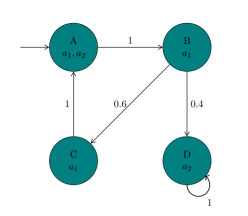
Sample Kripke structure (Hansson & Jonsson, 1994)
This sample structure K has 4 states: A, B, C, and D
K also has 5 transitions (i.e. labelled directed edges with non-zero probability): A → B, B → C, B → D, D → D, C → A)
The initial state is A, labelled with { a1, a2 }
There is a feedback loop for state D, labelled with { a2 }
There is a directed cycle leading from state A through B and C back to A
NOTE: Both the feedback loop for D and the directed cycle (A → B → C → A) would be disallowed in DAGs and the Pearl Causal Model
IMPLICATION: The Kleinberg Causal Model, with its reliance on probabilistic Kripke structures, is more expressive
Prima Facie & Genuine Causes
Test for causal significance
Under the Kleinberg Causal Model, where c and e are PCTL formulae, c is a prima facie cause of e if there is a p such that the following conditions are satisfied:
CONDITION 1:
F≤∞>0c
A state where c is true will finally be reached with non-zero probability
CONDITION 2:
c ⟿ ≥1,<∞≥pe
The probability of reaching a state where e is true (within the time bounds), after being in a state where c is true, is ≥p
CONDITION 3:
F≤∞<pe
The probability of reaching a state where e is true, after simply starting from the initial state of the system, is <p
Where CONDITIONS 1-3 are satisfied, c may be identified as a prima facie cause of e
Let X denote the set of prima facie causes of e
Let εx(c, e) = P(e|c ∧ x) − P(e|∼c ∧ x)
εavg(c, e) denotes the significance of cause c for an effect e
One computes εavg(c, e) by summing across the values of εx(c, e) for all members of X except c and dividing by the number of prima facie causes besides c
Just so causes are prima facie causes whose εavg is greater than the threshold
∴ The Kleinberg Causal Model considers each prima facie cause w.r.t. other prima facie causes, in order to determine genuine causes
Problems with the Kleinberg Causal Model
Problems with the Kleinberg Causal Model
Problem
Description
PROBLEM 1: Incompleteness w.r.t. All Relationships
Kleinberg's method is not intended as a method for recognizing all the possible manifestations of causality
If a relationship cannot be represented by PCTL, then it lies outside the scope of the Kleinberg Causal Model
PROBLEM 2: Incompleteness w.r.t. Epistemic States
We cannot represent people's intentions or states of knowledge under the Kleinberg Causal Model, although these epistemic states may be causally efficacious
∴ Kleinberg (2013) anticipates the extension of her method to include beliefs
PROBLEM 3: Data Quality
The Kleinberg Causal Model requires the development of strategies for combining diverse data sources at multiple scales (e.g. from populations to individuals to cells) and levels of granularity
PROBLEM 4: Need for Corroboration
There is nearly always a need for corroboration through other methods (viz. using background knowledge, conducting experimental studies, etc)


