When one particular species of event has always … been conjoined with another,
we make no longer any scruple of foretelling one upon the appearance of the other,
and of employing that reasoning, which can alone assure us of any matter of fact or existence.
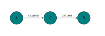
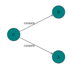
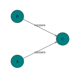
We then call the one object, Cause; the other, Effect.
- David Hume's (1748, §7) An Enquiry Concerning Human Understanding
Pearl Causal Model
|
|||||||||||||
|---|---|---|---|---|---|---|---|---|---|---|---|---|---|
Graph Theory |
|||||||||||||


|
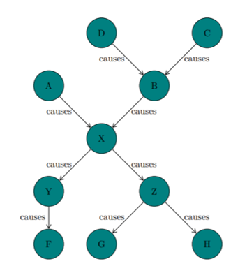
Relative to GRAPH 1: The parents of X are A and B The ancestors of X are D, C, A, and B The children of X are Y and Z The descendants of X are Y, Z, F, G, and H The indegree of X is 2 The outdegree of X is 2 The degree of X is 4
|
||||||||||||
D-separation |
|||||||||||||

|
The rules for d-separation (Pearl, 1988): RULE 1 for d-separation ('d' stands for 'directional'): X and Y are d-connected if there is an unblocked path between X and Y An unblocked path is a path that can be traced without meeting with any colliders 
In EXAMPLE 1: There is a collider at T The path X-R-S-T is unblocked ∴ X and R, X and S, X and T, R and S, R and T, and S and T are d-connected The path T-U-V-Y is also unblocked ∴ T and U, T and V, T and Y, U and V, U and Y, and V and Y are also d-connected However, X and Y, X and V, S and U, etc are d-separated: no path can be traced between them without meeting the collider at T RULE 2 for d-separation: X and Y are d-connected, conditioned on a set Z of nodes, if there is a collider-free path between X and Y that does not traverse any members of Z 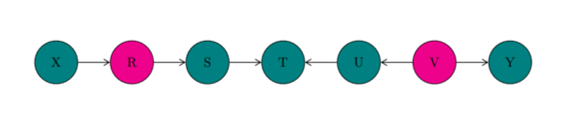
In EXAMPLE 2: Let Z be the set { R, V } According to RULE 2: X and S are d-separated: the path X-R-S is blocked by Z U and Y are d-separated: the path U-V-Y is blocked by Z S and U are d-separated: the path S-T-U is not collider-free Although T is not in Z, the path S-T-U is still blocked since T is a collider (RULE 1) RULE 3 for d-separation: If a collider is a member of the conditioning set Z or the collider has a descendant in Z, then it no longer blocks any path that traces this collider 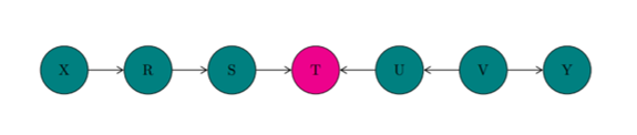
In EXAMPLE 3: Let Z be the set { T } According to RULE 3: X and Y, X and V, S and U, etc are now d-connected, since the collider T is a member of the conditioning set Z (compare with EXAMPLE 1) 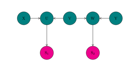
In EXAMPLE 4: Let Z be the set { S1, S2 } According to RULE 3: The collider at U has a descendant S1 in the conditioning set Z and the link at U is unblocked The collider at W has a descendant S2 in the conditioning set Z and the link at W is unblocked ∴ We now have a collider-free path between X and Y (viz. X-U-V-W-Y) that does not traverse any members of the conditioning set Z There are 3 blocking criteria:
A d-separated (or blocked) path does not transmit association A d-connected (or unblocked) path may transmit association |
||||||||||||
DAGs & Bayesian Networks |
|||||||||||||
|
The Pearl Causal Model takes a set of data and produces a directed acyclic graph (DAG) A DAG is:
A DAG is also called a Bayesian network (BN) The DAG represents the causal structure of the system Conditional dependence relations between variables are represented as edges between vertices in the graph The main idea behind the Pearl Causal Model is to find a graph or set of graphs that best explain the data There are two primary METHODS for inferring BNs from the data: METHOD 1: Assign scores to graphs and search over the set of possible graphs, while attempting to maximize a particular scoring function An initial graph is generated in METHOD 1 and the search space is explored by altering this graph METHOD 2: Start with an undirected, fully connected graph and use repeated conditional independence tests to remove and orient edges in the graph After the edges are removed, the remaining ones are directed from cause to effect 
Image source: Wikipedia Dynamic Bayesian networks (DBNs) use BNs to show how variables influence each other across time (Friedman et al, 1998, Murphy, 2002)
|
||||||||||||
Axioms |
|||||||||||||

|
AXIOM 1: Causal Markov Condition (CMC) A directed acyclic graph (DAG) G over V and a probability distribution P(V) satisfies the CMC iff for every W in V, W is independent of its non-effects, given its parents (Alternatively) Given any disjoint sets A, B, and C of variables, if A is d-separated from B conditional on C, then A is statistically independent of B given C See Pearl (1988) for proof Formally: W ⫫ { V \ Descendants(W) ∪ Parents(W) }|Parents(W) 
In EXAMPLE 5: The CMC entails the following conditional independence relations: A ⫫ B D ⫫ { A, B }|C
AXIOM 2: Causal Faithfulness Condition (CFC)
Given any graph, the CMC (or AXIOM 1) determines a set of independence relations However, a probability distribution P on a graph G that satisfies the CMC may include other independence relations besides those entailed by the CMC Recall the birth control pill EXAMPLE (Hesslow, 1976, Cartwright, 1989): 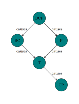
BCP (birth control pills) and T (thrombosis) might be independent in the probability distribution satisfying the CMC for this graph, even though the graph does not entail their independence ∴ If all and only those conditional independence relations true in P are entailed by the CMC applied to G, then we say that P and G are faithful to one another (Alternatively) Given any disjoint sets A, B, and C of variables, if A is statistically independent of B given C, then A is d-separated from B conditional on C
AXIOM 3: Causal Sufficiency
A set V of variables is causally sufficient for a population iff in the population every common cause of any 2 or more variables in V is in V According to AXIOM 3, there are no hidden common causes |
||||||||||||
Intervention & the Do-calculus |
|||||||||||||


|
EXAMPLE: Here is the DAG for the relationship between temperature, ice cream sales, and crime rates: 
X denotes ice cream sales Y denotes crime rates Z denotes the temperature UX, UY, and UZ denote the error terms for X, Y, and Z (i.e. the effects of exogenous variables not included in the causal model Suppose that we intervene on the value of ice cream sales (X) We might fix the value of X to a low value (e.g. by shutting down all ice cream shops) 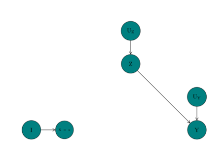
When we intervene on X:

According to the do-calculus: Given 2 disjoint sets of variables X and Y, the causal effect of X on Y is a function from X to the space of probability distributions on Y The causal effect of X on Y is denoted as 'P(y | do(x))' in the do-calculus For each realization x of X, P(y | do(x)) gives the probability of Y = y induced by deleting from the model all equations corresponding to variables in X and substituting X = x in the remaining equations The graph corresponding to the reduced set of equations is the subgraph from which all directed edges entering X have been pruned by surgery Where x1, …, xn denote variables in a BN: P(x1, …, xn) = ∏ P(xi|Parents(xi) According to Cochrane's EXAMPLE (Wainer, 1989): Soil fumigants (X) are being used to increase oat crop yields (Y) by controlling the eelworm population (Z) 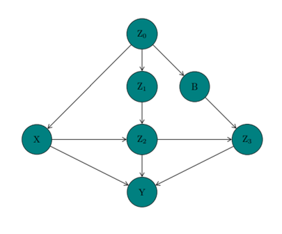
X denotes the soil fumigants Y denotes the oat crop yields Z denotes the eelworm population: Z0 denotes last year's eelworm population, Z1 denotes the quantity of eelworm population before treatment, Z2 denotes the quantity of eelworm population after treatment, and Z3 denotes the quantity of eelworm population at the end of the season B denotes the population of birds and other predators From P(x1, …, xn) = ∏ P(xi|Parents(xi), we get: P(z0, x, z1, b, z2, z3, y) = P(z0)P(x|z0)P(z1|z0)P(b|z0) × P(z2|x, z1)P(z3|z2, b)P(y|x, z2, z3) With the intervention do(X = x′): P(z0, z1, b, z2, z3, y|do(X = x′)) = P(z0)P(z1|z0)P(b|z0) × P(z2|x′, z1)P(z3|z2, b)P(y|x′, z2, z3) |
||||||||||||

Background image taken from: https://cdn.asiatatler.com/asiatatler/i/th/2020/02/04101225-aurora-1185464-1920_cover_1920x1280.jpg This website has been coded using html, css, and js and is dedicated to B and H .