When one particular species of event has always … been conjoined with another,
we make no longer any scruple of foretelling one upon the appearance of the other,
and of employing that reasoning, which can alone assure us of any matter of fact or existence.
We then call the one object, Cause; the other, Effect.
- David Hume's (1748, §7) An Enquiry Concerning Human Understanding
Granger Causality
Recall the various philosophical theories of causation:
The regularity theory of causation — C causes E if every event of type C is followed by an event of type E
The counterfactual theory of causation — C causes E iff E is causally dependent on C or there is a chain of causal dependence between C and E (analyzed in terms of counterfactual dependence)
The probabilistic theory of causation — C causes E iff C alters the probability of E
PROBLEMS with these philosophical theories of causation:
PROBLEM 1: Lack of philosophical consensus about the concept of causality
'Unlike art, causality is a concept whose definition people know what they do not like but few know what they do like' (Granger, 1980)
PROBLEM 2: Lack of usefulness in philosophical contributions to causality
See Hart & Honoré (1959) for a discussion on the lack of usefulness of the philosophers' contribution to causality
PROBLEM 3: Lack of common usage terms in philosophical discussions about causality
According to Granger (1980, p. 331), philosophers make no attempt to use common usage terms in their discussion
PROBLEM 4: Lack of concern with operational definitions
Philosophers are not constrained to look for operational definitions
Conversely, the primary advantage of the Wiener-Granger causality approach is that it is easy to understand and pragmatic (see Granger, 2007, pp. 290-1, 294)
For Granger (1980), the ultimate objective is to produce an operational definition of causality
CAVEAT:
There is a difference between Granger causality and the common-sense understanding of the cause-effect relationship (Lin & Bahadori, 2012)
In addition, Granger's definition of Granger causality has been debated in both philosophy (Cartwright, 1989) and economics (Chowdhury, 1987, Jacobs et al, 1979)
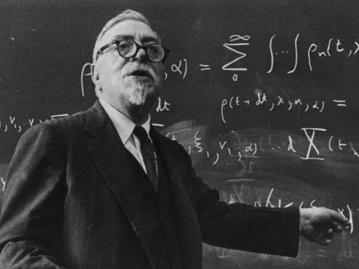
Norbert Wiener
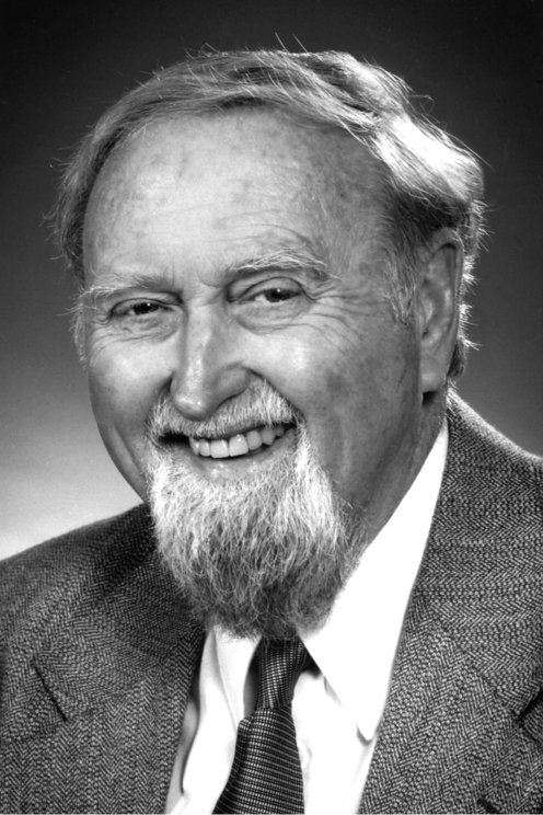
C. W. J. Granger
According to Wiener (1956, p. 127):
For 2 simultaneously measured signals, if we can predict the 1st signal better by using the past information from the 2nd signal than by using the information without it, then we call the 2nd signal causal to the 1st one
According to Granger (1980, p. 334):
Let A and B denote two time-series variables
A Granger-causes B, if the probability of B conditional on its own history and the history of A (beside the set of available information) does not equal the probability of B conditional on its own history alone
∴ This statistical approach to causality is known as Wiener-Granger causality, since Granger's work built on ideas from Wiener (1956)
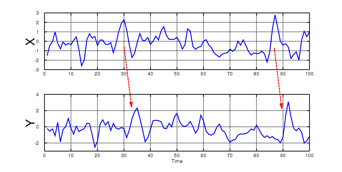
Granger (1969, 1980) developed a statistical method to take two time series and determine whether one is useful for forecasting the other
Time series X Granger-causes time series Y
Image source: Wikipedia
Granger did not attempt to relate his method to philosophical definitions of causality
Rather, Granger proposed a new definition of Granger causality that is most similar to correlation
EXAMPLE (Granger, 1980):
Suppose that X and Y are the only two random variables in the universe
Suppose further that a strong correlation is observed between X and Y
Suppose in addition that God (or an acceptable substitute) can confirm that X does not cause Y
This leaves open the possibility of Y causing X
∴ The strong observed correlation between X and Y might lead to the acceptance of the claim that Y causes X
Formal definition of Granger causality:
Let Xt and Yt denote two variables that are suspected to be causally related
Let Ωt denote all the knowledge available in the universe at t
Xt Granger-causes Yt + 1 iff:
P(Yn + 1 ∈ A | Ωn) ≠ P(Yn + 1 ∈ A | Ωn − Xn) for some A
TRANSLATION: In order for causation to occur, the variable Xn(i.e. the values of variable X up to time n) needs to have some unique information about the value that Yn + 1 (i.e. the value of variable Y at time n + 1) will take in the immediate future
Axioms
Image source: Eric Sucar
The axioms of the Wiener-Granger causality approach:
AXIOM 1: The past and the present may cause the future, but the future cannot cause the past
While the truth of AXIOM 1 cannot be tested using the methods discussed by Granger (1980), work by physicists on time-reversibility does not seem to contradict AXIOM 1 (see Overseth (1967))
AXIOM 2: Ωn contains no redundant information, where Ωn denotes all the knowledge available in the universe at n
If some variable Zn is functionally related to one or more other variables in a deterministic fashion, then Zn should be excluded from Ωn
EXAMPLE:
Temperature can be measured hourly at some location in both degrees Fahrenheit (°F) and degrees Centigrade (°C)
There is no point in including both these variables in Ωn
AXIOM 3: All causal relationships remain constant in direction throughout time
While the strength and lag of causal relationships may change, causal laws are not allowed to change from positive strength to zero, or go from zero to negative strength, through time
IMPLICATIONS of AXIOMS 1-3:
IMPLICATION 1:
Feedback loops are not ruled out: if Xn causes Yn + 1 w.r.t. some information set, then this implies no restrictions on whether or not Yn causes causes Xn + 1
IMPLICATION 2:
It is impossible to find a cause for a series that is self-deterministic: that variable is perfectly forecastable from its own past
IMPLICATION 3:
Instantaneous causality: if there is a data collection problem, then both Xt and Yt could have a common cause that is not included in the information set
IMPLICATION 4:
Spurious causation: where Zt is the common cause of both Xt and Yt, there may be a spurious causation of Y by X if the information set is too restricted
The spurious causation of Y by X w.r.t. the information set Jn(X, Y) vanishes when the information set is expanded to include Z
Tests
TEST 1: Bivariate Granger test
Only two time-series are included: the cause Yt and the effect Xt
TEST 1 is concerned with whether Y causes X w.r.t. the information set Jn(X, Y) (i.e. the two-variable case) (Pierce & Haugh, 1977)
TEST 2: Multivariate Granger test
TEST 2 includes other variables in the model of each time series
TEST 2 comes closer to causal inference than the bivariate test
PROBLEMS with TESTS 1 & 2
Test
Problem
TEST 1 (Bivariate)
PROBLEM 1: TEST 1 does not capture Granger's original definition of Granger causality
Ωn (i.e. all the knowledge in the universe available at time n) is multivariate and Yn (i.e. the values taken by the variable Y up to time n) could be multivariate
PROBLEM 2: TEST 1 cannot distinguish between causal relationships and correlations between effects of a common cause
TEST 2 (Multivariate)
PROBLEM 1: Computational complexity
TEST 2 becomes computationally infeasible with even a moderate number of lags and variables
Many areas of work involve influence over long periods of time (e.g. epidemiological studies), but these would be prohibitively complex to test
More generally:
PROBLEMS with the Wiener-Granger causality approach
PROBLEM 1: Granger causality ≠ Causality
The Wiener-Granger causality approach aims to infer relationships between time series
However, Granger causality is not generally considered to be a definition of causality or a method of its inference
There is a plurality of statistical tests (e.g. the Granger direct test, the Sims test, etc) associated with the Wiener-Granger causality approach
∴ It is possible to apply two distinct Granger-causality tests T1 and T2 w.r.t. the same dataset and obtain different outcomes
For instance, T1 could confirm the null hypothesis while T2 might reject the null hypothesis
This contradicts AXIOM 3, according to which all causal relationships must remain constant in direction throughout time
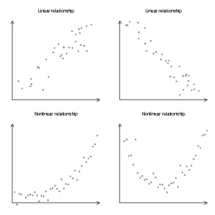
PROBLEM 3: Nonlinear causal relationships
The most popular tests (e.g. General Granger causality test, Sims test, modified Sims test) associated with the Wiener-Granger causality approach were developed to test only for linear dependencies
∴ One may mistakenly interpret the failure of a test to reject the null hypothesis as evidence for a lack of causality, when there may in fact be a nonlinear causal relationship
PROBLEM 4: Sampling frequency
When the sampling frequency is insufficient, test results may show bidirectional Granger causality, although the real, unidirectional causal relationship exists and can be detected
PROBLEM 5: Rational expectations
EXAMPLE:
Suppose that a company C is able to predict inflation I rationally (e.g. using better information)
C then makes purchases X whose amount depends on a future rise in prices and storage cost
∴ The expected causal relationship would have the opposite direction: It + 1 Granger-causes Xt
This would violate AXIOM 1, according to which the future cannot cause the past
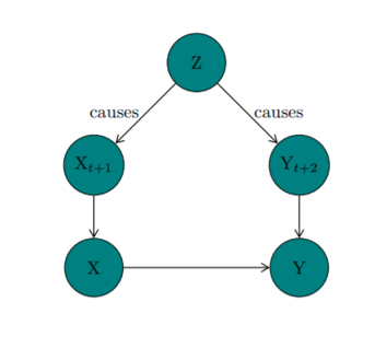
PROBLEM 6: Common causes
EXAMPLE:
Z is the common cause of Xt + 1 and Yt + 2
To an observer, it will appear (erroneously) to be the case that Xt + 1 Granger-causes Yt + 2
The common cause fallacy should be suspected when Granger causality tests indicate bidirectional Granger causality (viz. X → Y and Y → X)
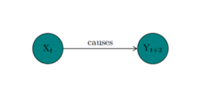
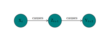
PROBLEM 7: Indirect causality
EXAMPLE 1: Direct causality
EXAMPLE 2: Indirect causality
Standard tests associated with the Wiener-Granger causality approach only show dependencies present within a time period and will be unable to distinguish between EXAMPLE 1 and EXAMPLE 2
Table of erroneous conclusions from Granger causality tests (Maziarz, 2015, p. 101)
The real causal relationship
X → Y
Y → X
X ⟷ Y
X ∅ Y
The test result
X → Y
CORRECT
Rational expectations (Noble, 1982)
Sampling frequency (McCrorie & Chambers, 2006)
Spurious causation due to nonlinear data
Sampling frequency
Common cause fallacy (Chu et al, 2004)
Y → X
Rational expectations (Noble, 1982)
CORRECT
Sampling frequency (McCrorie & Chambers, 2006)
Spurious causation due to nonlinear data
Sampling frequency
Common cause fallacy (Chu et al, 2004)
X ⟷ Y
Sampling frequency
Sampling frequency
CORRECT
Common cause fallacy (Sims, 1977)
X and Y may be determined by a 3rd variable Z
X ∅ Y
Causal relationship is nonlinear
Indirect causality (Dufour & Taamouti, 2010)
Causal relationship is nonlinear
Indirect causality (Dufour & Taamouti, 2010)
Time series are non-stationary (Glasure & Lee, 1998)
CORRECT
KEY:
→ denotes unidirectional Granger causality
⟷ denotes bidirectional Granger causality
∅ denotes no causal relationship
Uses
The Wiener-Granger causality approach is the most influential approach to causality in economics (Hoover, 2006)
Granger causality is now being applied to econometrics, finance (Granger, 2007), neuroscience (Bressler & Seth, 2011, Ding et al, 2006), epidemiology, and physics to model information flow


