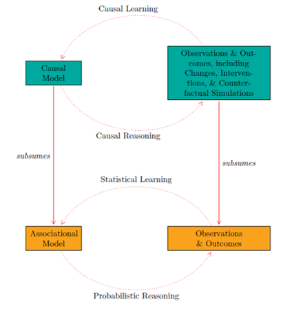
FIG. 1:
Association vs. Causation.
Adapted from Peters et al (2017) |
P1: Association is generally a good guide to causation.
P2: However, association is no guarantee of causation.
P1 and P2 are normally taken for granted in statistics primers.
There are two ways to determine the causal effect of one variable on another:
OPTION 1: Experimentation and measurement of causal effects
OPTION 2: Observation and estimation of causal effects relative to the observational dataset
|
Randomized Controlled Trials (RCTs) are supported by Fisher's (1925) theory of experimental design
RCTs rely on randomization (e.g. allocating members of a sample population into either the Treatment Group or the Control Group with the toss of a fair coin) to eliminate bias
However, it is often infeasible or impossible to conduct RCTs
∴ We may have to consider OPTIONS 2A-2C instead |
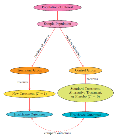
FIG. 2:
Randomized Controlled
Trials (RCTs)
(OPTION 1)
|

FIG. 3:
The Logic of Counterfactuals
(OPTION 2A) |
The Logic of Counterfactuals has been developed by philosophers:
i) Robert Stalnaker (1968)
ii) David Lewis (1973)
The Logic of Counterfactuals relies on the Semantics of Possible Worlds
|
The Rubin Causal Model or Potential Outcomes Approach has been developed by statisticians like:
i) Donald Rubin (1974)
ii) James Robins (1986)
iii) Miguel Hernán and James Robins (2020)
The Rubin Causal Model or Potential Outcomes Approach relies on a set of Identifiability Conditions:
a) The Consistency Condition: the treatment is well-defined
b) The Exchangeability Condition: the conditional probability of receiving treatment T depends only on the measured covariates L
c) The Positivity Condition: the probability of receiving any value of treatment conditional on L is positive
|

FIG. 4:
The Potential Outcomes Approach
(OPTION 2B) |

FIG. 5:
The Do-Calculus Approach
(OPTION 2C) |
The Do-Calculus Approach has emerged from computer science as a result of the groundbreaking work of Judea Pearl (2000)
The Do-Calculus Approach relies on such axioms as the Causal Markov Condition and the Causal Faithfulness Condition:
a) The Causal Markov Condition: for every node W in a set of nodes V, W is independent of its non-effects, given its parents
b) The Causal Faithfulness Condition: if all and only those conditional independence relations true in the probability distribution P are entailed by the Causal Markov Condition applied to a graph G, then P and G are faithful to one another
|
Whether we go for OPTION 2A, OPTION 2B, or OPTION 2C, we will still have to adjust for confounders
Confounders are a set of measured covariates listed under node L (see FIG. 6) that affect the values of both treatment T and healthcare outcome Y
In our Medical AI project, we rely on the domain-specific expertise of our medical collaborators to identify possible confounders
|
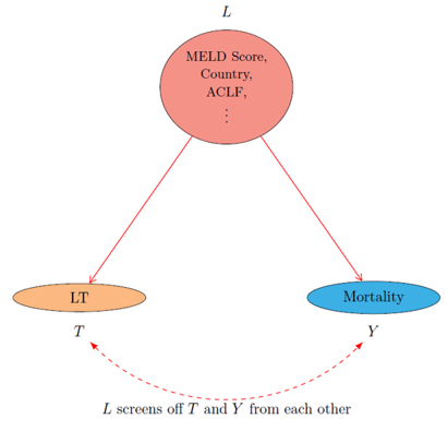
FIG. 6:
Dealing with Confounders |